Note: Most of this work was completed in 2014. These results may not hold with current drivers and more recent hardware (e.g., Carrizo)
Kaveri is AMD's first APU (accelerated processing unit, e.g. a chip with both a CPU and GPU on-die) to provide an implementation of heterogeneous system architecture (HSA). HSA is set of standards from the HSA Foundation which provides transparent support for multiple compute platforms. The goal is to allow programmers to use the GPU to accelerate parts of their applications with minimal overhead, both in terms of performance overhead and programmer effort.
The key features which differentiate HSA from other similar technologies are
- Shared virtual memory which allows the CPU and GPU to access the same data transparently.
- Heterogeneous queuing which allows the user-mode program to offload work to the GPU without OS intervention. Also, it allows CPU to schedule work for the GPU, the GPU to schedule work for the CPU, the GPU to schedule work for itself, etc.
- Architected signals and synchronization which is mostly used for implementing the heterogeneous queues, but also allows for complex asynchronous communication between different compute platforms.
There are many questions about how AMD has implemented these features in their first iteration of HSA hardware. In this post, I am going to focus on the implementation of shared virtual memory.
Deducing Cache Parameters
There is a great paper from the early 90's which looks at several machines available at the time and determines their cache parameters. Apparently, back then, we didn't have resources like Intel's architecture pages which gives us at least some information on what is in a manufactured chip. The paper by Saavedra et. al (available here) presents a simple microbenchmark (described below) and formulas which take the runtime of the benchmark and tell you the cache parameters.
This table is an overview of my findings. Below, I detail the methods and data that lead to these results. Information in italics I'm less sure about than the rest of the data.
| Capacity | Miss Latency | Associativity | |
|---|---|---|---|
| L1 Cache | 16 KB (Per CU) | 225 ns | 64-way |
| L2 Cache | 256 KB (8 32 KB banks) | 50 ns | at least 64-way |
| L1 TLB | 64MB-128MB reach 64-128 2MB entries 2046 32 KB or 64 2 MB entries | 450 ns | at least 64-way |
| L2 TLB (none if 2MB pages) | 512 MB reach 256 2 MB entries | 220 ns | 256-way (for 4K pages) |
The microbenchmark
(note: the code used to generate the data in this notebook and the data itself can be found on github.)
The microbenchmark that I used is quite simple. It allocates a chunk of memory, then issues memory requests to that memory. By varying the amount of memory allocated and the stride between each memory access, you can control the cache's effect. For instance, if the size of the allocated memory is less than or equal to the cache size, we would expect the entire array to fit in the cache and every access to hit in the cache, experiencing only the cache hit latency. Alternatively, if the allocated memory was larger than the cache, and we used a stride equal to the cache line size, we would expect every access to miss in the cache, experiencing the cache miss latency on every access.
Although the benchmark is simple, things are complicated by prefetching, multi-level caches, TLBs, replacement policies, etc. Some of these are relatively easy to overcome (we can trick the prefetcher by pointer chasing, for instance). Other things, like replacement policies other than LRU, cause the data to be more noisy or to not follow the model laid out by Saavedra et. al exactly.
In the data below, I've tried to explain as much as I can about why we see the data, but there are still some holes in my understanding.
The data!
For each of the graphs below, I've run the microbenchmark with input arrays from 4 KB up to 4 GB and strides from 4 bytes to the size of the array.
Baseline data
This first set of data uses the GPU to initialize the data (i.e. the data is touched by the GPU before the test is performed). It also uses the default Linux allocator, which uses transparent huge pages (THP) in this case.
data = pd.read_csv(urlbase+'data-thp-gpu.csv', usecols=(4,5,6), skipinitialspace=True)
figure(figsize=(12,6.66))
title('Init on GPU with THP')
for i in range(12,33):
    plt(2**i, data=data)
legend(loc='upper right')
xscale('log', basex=2)
grid(b=True, which='major')
xlabel('stride')
ylabel('time (ns)')
annotTHP()
tight_layout()
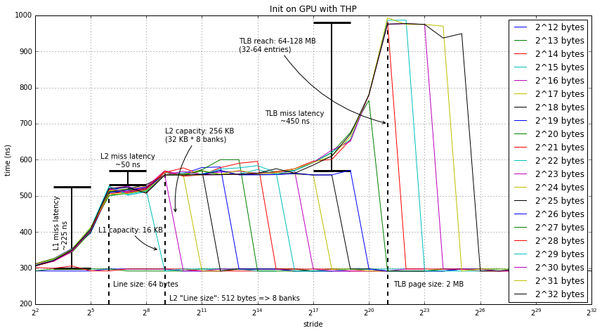
Starting on the left (and with smaller inputs):
- The first array size which experiences L1 misses (the first teal
line) is 215
- This implies that the L1 cache capacity is < 32 KB, likely 16 KB.
- Since the latency changes from 300ns to 525ns, we can also infer that the L1 miss latency is 225ns. This may seem like a very high miss latency; however, it's not out of the realm of possibility for GPU caches. I've found similar numbers for both NVIDIA and AMD discrete GPUs.
- Also, the stride at which the latency is a maximum for the 215 line is 64 bytes, which implies a 64 byte line. The reason we know it's the line size is that until we stride at the line size or above, the cache misses are partially amortized by hitting multiple times within the same cache block.
- Next, the next array size (216) seems to have a
significantly different latency for each access.
- I believe this is the L2 miss latency, which is much smaller than the L1 miss latency at only 50ns. I assume that this L2 miss latency is actually the DRAM latency. If this is the case, the 50ns is quite reasonable. In discrete GPUs, the DRAM latency is much higher, but 50ns is reasonable for DDR3.
- However, I do not believe that the L2 cache is only 32 KB. It wouldn't make much sense to include if it was so small. What I believe is going on here (and I've yet to develop a test to confirm this hypothesis) is that the L2 has a 512 byte "line size", or as it's likely implemented, 8 banks and the banks are addressed by simple address slicing. If this is true, then the L2 is actually 256 KB, a much more reasonable size.
- Nothing else interesting happens until we get to arrays larger than
227. At this point, we start missing in another level of
cache. It's likely that this "cache" is actually the TLB.
- Since there is an increase in latency for 227 and it doesn't level off until 228, it is likely the TLB reach is between these two sizes (64 MB and 128 MB).
- Looking at the 228 line, and the ones after it, we see that latency levels off after a stride of 221 or 2 MB. Interestingly, this is the large page size for x86-64. Thus, it seems that the GPU is using huge pages... cool!
- If we use this page size of 2 MB, then the 64 MB to 128 MB reach implies that the TLB has 32 to 64 entries. This is quite reasonable for a modern TLB. An interesting question is whether this TLB is local to the compute unit, or if it's shared between many compute units on the GPU. This could be the local TLB, or it could be the IOMMU TLB.
- Finally, we can see that the TLB miss latency is quite large, almost 500ns. Again, this is quite reasonable, especially if we assume that a TLB miss will take 1-4 memory accesses. (Well, 1-3 in this case since the GPU is using 2 MB pages).
GPU data without THP
Next we are going to look at what happens with the same test if we disable THP. This forces the GPU to use 4 KB pages. Though, interestingly, looking at the data, the GPU uses 32 KB pages even though the underlying page size is 4 KB!
Let's look at the data. It's generated using exactly the same methods as before.
data = pd.read_csv(urlbase+'data-nothp-gpu.csv', usecols=(4,5,6), skipinitialspace=True)
figure(figsize=(12,6.66))
title('Init on GPU without THP')
for i in range(12,33):
    plt(2**i, data=data)
legend(loc='upper right')
xscale('log', basex=2)
grid(b=True, which='major')
xlabel('stride')
ylabel('time (ns)')
annotNoTHP()
tight_layout()
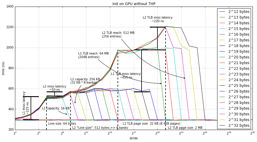
Most of this data is the same as when using THP. The main difference is that we can see TLB misses with a much small array than in the previous data and that there are two TLB "line sizes".
- Looking at the first level TLB, we see the line size is 32 KB. This actually isn't that strange of a "page" size. It's 8 4 KB pages, which happens to be the number of page translations that can fit in one 64 byte cache line. My hypothesis is that the GPU is using something like a sub-blocked TLB.
- Interestingly, this TLB seems huge (2048 32 KB entries), especially if we compare it to the TLB in the first data. Since it's so big, my guess is that it's at the IOMMU and shared by the whole GPU, not a per-CU TLB. Additionally, there may be more sub-blocking going on all the way up to the 2 MB page size. Sub-blocking up to 2 MB pages lines up with the previous THP data the best. If the used 2 MB super-blocks then it would have 64 entries, which lines up with the L1 TLB in the previous data (which we found to be 64-128 entries).
- Next, we again see the 2 MB page, but this time only for arrays larger than 512 MB. I find this quite strange that we didn't see this level of TLB in the previous data that had only 2 MB pages. It seems that this "L2 TLB", whatever it is, has an additional miss penalty not seen in the previous data. Assuming this TLB uses 2 MB pages, then it would have 256 entries.
I'm honestly not too sure what exactly is going on here. The data is pretty clear that there's two levels of TLB, but I'm not sure how these TLB levels relate to the TLB in the first set of data with 2 MB pages.
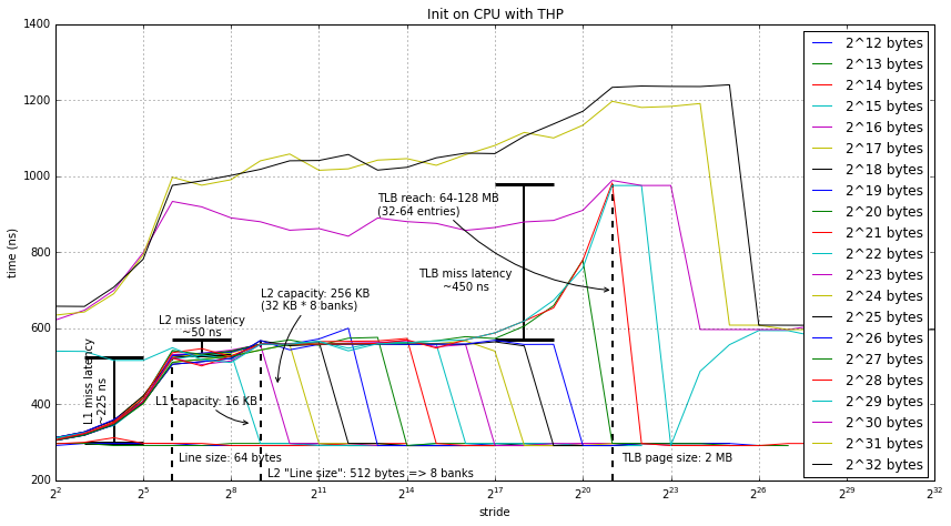
CPU first touch
Next, we're going to look at what happens when the GPU doesn't touch the data before the test is performed. For this test, I used the CPU to initialize the data and then performed the test on the GPU. Below we have the data both when THP is enabled and disabled. Since there aren't too many new data points in these two graphs I'll talk about them together below the graphs.
data = pd.read_csv(urlbase+'data-thp-cpu.csv', usecols=(4,5,6), skipinitialspace=True)
figure(figsize=(12,6.66))
title('Init on CPU with THP')
for i in range(12,33):
    plt(2**i, data=data)
legend(loc='upper right')
xscale('log', basex=2)
grid(b=True, which='major')
xlabel('stride')
ylabel('time (ns)')
annotTHP()
tight_layout()
data = pd.read_csv(urlbase+'data-nothp-cpu.csv', usecols=(4,5,6), skipinitialspace=True)
figure(figsize=(12,6.66))
title('Init on CPU without THP')
for i in range(12,33):
    plt(2**i, data=data)
legend(loc='upper right')
xscale('log', basex=2)
grid(b=True, which='major')
xlabel('stride')
ylabel('time (ns)')
annotNoTHP()
tight_layout()
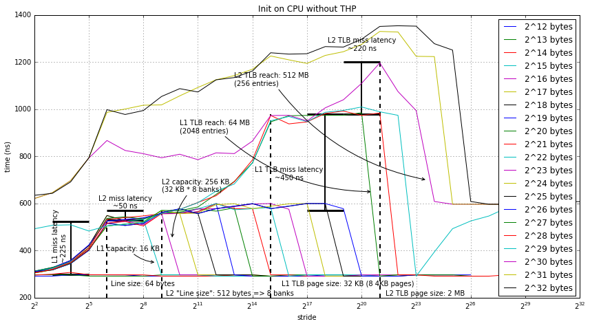
The key difference between these two graphs and the first two (where the data was first initialized on the GPU) is for arrays of sizes 512 MB and above we see some pretty strange data. The way I interpret this data, and I may be totally wrong about this, is that the GPU caches are disabled. I believe this is true because of the latency seen using the word (4 byte) stride. Even in this case, when you would expect to get intra-block hits, the latency equal to the cache miss latency.
Although disabling the GPU caches really hurts performance for this microbenchmark, it may make sense for real applications. Maybe the runtime is somehow detecting that the data is written by the CPU and assumes that if the GPU wants up to date data that the highest performance option is to disable the caches (rather than rely on cache coherence).
I have considered other possibilities, like 1 GB pages, page faults, etc. But I can't come up with any other reason other than the above for this data.
Conclusions
There are still many unanswered questions about the design of the caches in Kaveri. This post just scratches the surface. I think the most interesting things that I learned are some of the details of the GPU MMU on Kaveri. (This may be most interesting to me since it's in my domain ;)). Also, it seems that accessing large arrays on the GPU that are first touched by the CPU results in very low performance. Since initializing data on the CPU and then processing that data on the GPU is a common idiom today, programmers will have to be careful to not use large arrays if they want to get high performance with AMD's current architecture.
Below I've included all of the other code that's required to get things to work. Questions and comments can be directed to me (Jason Lowe-Power) at powerjg@cs.wisc.edu. I'd like to thank my advisers Mark Hill and David Wood for helpful discussions about this data.
Code for generating the above graphs:
def plt(size, data):
    d = data[data['size'] == size]
    plot(d['stride'], d['overall_kernel_time']/100/1024*1e9, label='2^%d bytes' % log2(size))

def annotNoTHP():
    # L1
    hlines(525, 2**3, 2**5, lw=3)
    hlines(300, 2**3, 2**5, lw=3)
    vlines(2**4, 300, 525, lw=2)
    text(2**3, 350, "L1 miss latency\n~225 ns", rotation=90, va='bottom')
    vlines(2**6, 200, 525, lw=2, linestyle='--')
    text(2**6+10, 250, "Line size: 64 bytes")
    annotate("L1 capacity: 16 KB", xy=(2**9-100,350), xytext=(2**5+2**4-5, 400),
             arrowprops=dict(arrowstyle="->",
                           connectionstyle="arc3,rad=.2"))

    # L2
    hlines(570, 2**6, 2**8, lw=3)
    hlines(530, 2**6, 2**8, lw=3)
    vlines(2**7, 530, 570, lw=2)
    text(2**7, 580, "L2 miss latency\n~50 ns", ha='center')
    vlines(2**9, 200, 570, lw=2, linestyle='--')
    text(2**9+100, 210, "L2 \"Line size\": 512 bytes => 8 banks")
    annotate("L2 capacity: 256 KB\n(32 KB * 8 banks)", xy=(2**9+2**8,450), xytext=(2**9, 650),
             arrowprops=dict(arrowstyle="->",
                           connectionstyle="arc3,rad=.2"))

    # L1 TLB
    hlines(980, 2**17, 2**19, lw=3)
    hlines(570, 2**17, 2**19, lw=3)
    vlines(2**18, 570, 980, lw=2)
    text(2**16, 700, "L1 TLB miss latency\n~450 ns", ha='center')
    vlines(2**15, 200, 980, lw=2, linestyle='--')
    text(2**15+2**14, 250, "L1 TLB page size: 32 KB (8 4KB pages)")
    annotate("L1 TLB reach: 64 MB\n(2048 entries)", xy=(2**20+2**19,650), xytext=(2**10, 900),
             arrowprops=dict(arrowstyle="->",
                           connectionstyle="arc3,rad=.2"))

    # L2 TLB
    hlines(1200, 2**19, 2**21, lw=3)
    hlines(980, 2**19, 2**21, lw=3)
    vlines(2**20, 980, 1200, lw=2)
    text(2**20, 1250, "L2 TLB miss latency\n~220 ns", ha='center')
    vlines(2**21, 200, 1200, lw=2, linestyle='--')
    text(2**21+2**19, 210, "L2 TLB page size: 2 MB")
    annotate("L2 TLB reach: 512 MB\n(256 entries)", xy=(2**23+2**22,700), xytext=(2**13, 1100),
             arrowprops=dict(arrowstyle="->",
                           connectionstyle="arc3,rad=.2"))

def annotTHP():
    # L1
    hlines(525, 2**3, 2**5, lw=3)
    hlines(300, 2**3, 2**5, lw=3)
    vlines(2**4, 300, 525, lw=2)
    text(2**3, 350, "L1 miss latency\n~225 ns", rotation=90, va='bottom')
    vlines(2**6, 200, 525, lw=2, linestyle='--')
    text(2**6+10, 250, "Line size: 64 bytes")
    annotate("L1 capacity: 16 KB", xy=(2**9-100,350), xytext=(2**5+2**4-5, 400),
             arrowprops=dict(arrowstyle="->",
                           connectionstyle="arc3,rad=.2"))

    # L2
    hlines(570, 2**6, 2**8, lw=3)
    hlines(530, 2**6, 2**8, lw=3)
    vlines(2**7, 530, 570, lw=2)
    text(2**7, 580, "L2 miss latency\n~50 ns", ha='center')
    vlines(2**9, 200, 570, lw=2, linestyle='--')
    text(2**9+100, 210, "L2 \"Line size\": 512 bytes => 8 banks")
    annotate("L2 capacity: 256 KB\n(32 KB * 8 banks)", xy=(2**9+2**8,450), xytext=(2**9, 650),
             arrowprops=dict(arrowstyle="->",
                           connectionstyle="arc3,rad=.2"))

    # TLB
    hlines(980, 2**17, 2**19, lw=3)
    hlines(570, 2**17, 2**19, lw=3)
    vlines(2**18, 570, 980, lw=2)
    text(2**16, 700, "TLB miss latency\n~450 ns", ha='center')
    vlines(2**21, 200, 980, lw=2, linestyle='--')
    text(2**21+2**19, 250, "TLB page size: 2 MB")
    annotate("TLB reach: 64-128 MB\n(32-64 entries)", xy=(2**21,700), xytext=(2**13, 900),
             arrowprops=dict(arrowstyle="->",
                           connectionstyle="arc3,rad=.2"))
urlbase = "https://raw.githubusercontent.com/powerjg/hsa-micro-benchmarks/master/caches/data/A10-7850K/"
import pandas as pd
Comments !